Relative positional embedding for any attention mechanism
In Shaw et al. (2018), the authors introduce relative positional embedding for self-attention in transformer models, and in Huang et al. (2018), the authors present a memory efficient approach to calculating this embedding in decoder blocks, in which the self-attention is causal. In this article, the approach is generalized to any attention mechanism, should it be self or cross or full or causal.
Background
The classical attention is formalized as follows:
\[A = \text{softmax}\left( \frac{QK^{T}}{\sqrt{n_d}} \right) V\]where \(K\), \(V\), and \(Q\) are the keys, values, and queries, respectively. The keys and values are of shape \(n_s \times n_h \times n_{t_1} \times n_d\) where \(n_s\) is the batch size (s for space), \(n_h\) is the number of attention heads, \(n_{t_1}\) is the window size (t for time) of the input sequence, and \(n_d\) is the head size. The queries are of shape \(n_s \times n_h \times n_{t_2} \times n_d\) where \(n_{t_2}\) is the window size of the output sequence.
The relative attention obtains one additional term in the numerator:
\[A = \text{softmax}\left( \frac{QK^T + S}{\sqrt{n_d}} \right) V. \tag{1}\]In the above, \(S\) is of shape \(n_s \times n_h \times n_{t_2} \times n_{t_1}\) and calculated based on \(Q\) and a matrix \(E\) of shape \(n_d \times n_{t_3}\) containing relative positional embeddings. The typical context is causal self-attention, in which \(n_{t_3}\) is thought of as the maximum allowed length of the input sequence and set to \(n_{t_1}\), with the interpretation that the embeddings are running from position \(-n_{t_1} + 1\) (the most distant past) up to \(0\) (the present moment). Then \(S\) is a specific arrangement of the inner products between the queries in \(Q\) and the embeddings in \(E\) so as to respect the arrangement in \(QK^T\).
The original and more memory efficient calculations of \(S\) in the case of causal attention, are illustrated in the figure below, which is taken from Huang et al. (2018).
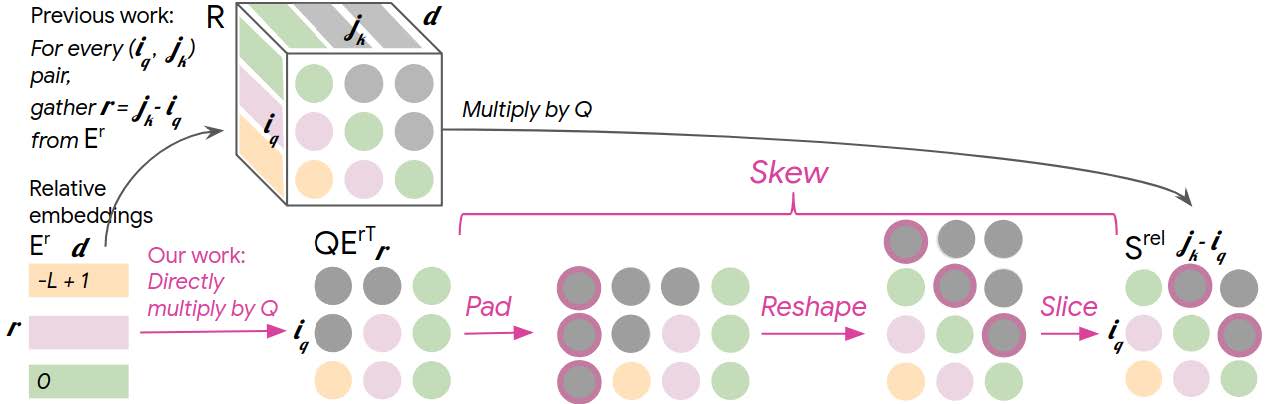
The matrix to the very right shows how \(S\) is arranged. Since the use case is causal attention, the upper triangle above the main diagonal (gray circles) is irrelevant and can contain arbitrary values, which it does in the algorithm proposed in Huang et al. (2018). The main diagonal (green circles) contains the inner products of the queries and the embedding corresponding to position \(0\). The first subdiagonal (pink circles) contains the inner products of the queries except for the first one as it has no past, and the embedding corresponding to position \(-1\). And it continues in this way down to \(-n_{t_1} + 1\), in which case it is only the last query that is involved, since it comes last in the sequence and has the longest past.
The calculation given in Huang et al. (2018) reduces the intermediate memory requirement from \(\mathcal{O}(n_h \, n_d \, n_t^2)\) to \(\mathcal{O}(n_h \, n_d \, n_t)\) where \(n_t\) is a general sequence length. However, it is limited to self-attention with causal connectivity, which is what is found in decoder blocks. It is not suitable for other attention patterns. Therefore, it cannot be used in, for instance, encoder blocks and decoder blocks with cross-attention, which usually have non-causal attention. In what follow, the limitation is lifted.
Algorithm
Let us extend \(E\) to be of shape \(n_d \times (2 n_{t_3} - 1)\) so that it has an embedding for any relative position not only when looking back in the past but also forward into the future, with \(n_{t_3}\) being the maximum allowed length of the input sequence as before, that is, \(t_1 \leq t_3\). Let us also interpret \(E\)’s columns as running from position \(n_{t_3} - 1\) (the most distant future) to position \(-n_{t_3} + 1\) (the most distant past). For instance, when the output sequence is of length \(t_3\) (the longest possible), the first query (position 0) will be “interested” only in columns \(0\) through \(n_{t_3} - 1\) inclusively, while the last (position \(n_{t_3} - 1\)) only in columns \(n_{t_3} - 1\) through \(2 n_{t_3} - 2\) inclusively.
Similarly to Huang et al. (2018), we note that multiplying \(Q\) by \(E\) results in a matrix that contains all the inner products necessary for assembling \(S\) in the general case. For instance, for \(t_3 = 4\) and dropping the batch and head dimensions for clearer visualization, the product is as follows:
\[QE = \left( \begin{matrix} s_{0 + 3} & s_{0 + 2} & s_{0 + 1} & s_{0 + 0} & & & \\ & s_{1 + 2} & s_{1 + 1} & s_{1 + 0} & s_{1 - 1} & & \\ & & s_{2 + 1} & s_{2 + 0} & s_{2 - 1} & s_{2 - 2} & \\ & & & s_{3 + 0} & s_{3 - 1} & s_{3 - 2} & s_{3 - 3} \\ \end{matrix} \right)\]where \(s_{i + t}\) denotes query \(i\) embedded to look at relative time \(t\), that is, the inner product between the query at position \(i\) and the embedding corresponding to a relative attention shift of \(t\), whose embedding is stored in column \(n_{t_3} - 1 - t\) of \(E\). For instance, for \(s_{2 - 1}\) with \(t_3 = 4\) still, the inner product is between row \(2\) of \(Q\) and column \(4 - 1 - (-1) = 4\) of \(E\).
The target arrangement is then simply the one where we stack the “interesting” diagonals of \(QE\) on top of each other from diagonal \(0\) (the main diagonal) at the bottom and diagonal \(t_3 - 1\) (the rightmost relevant superdiagonal) at the top
\[\bar{S} = \left( \begin{matrix} s_{0 + 0} & s_{1 - 1} & s_{2 - 2} & s_{3 - 3} \\ s_{0 + 1} & s_{1 + 0} & s_{2 - 1} & s_{3 - 2} \\ s_{0 + 2} & s_{1 + 1} & s_{2 + 0} & s_{3 - 1} \\ s_{0 + 3} & s_{1 + 2} & s_{2 + 1} & s_{3 + 0} \\ \end{matrix} \right)\]and then transpose the result
\[S = \left( \begin{matrix} s_{0 + 0} & s_{0 + 1} & s_{0 + 2} & s_{0 + 3} \\ s_{1 - 1} & s_{1 + 0} & s_{1 + 1} & s_{1 + 2} \\ s_{2 - 2} & s_{2 - 1} & s_{2 + 0} & s_{2 + 1} \\ s_{3 - 3} & s_{3 - 2} & s_{3 - 1} & s_{3 + 0} \\ \end{matrix} \right).\]More generally, the algorithm can be summarized as follows:
\[S = \text{transpose}\left( \text{diagonal}\left( QE, \, \text{lower}=0, \, \text{upper}=n_{t_3} - 1 \right) \right)\]where \(\text{diagonal}\) is a function taking a tensor and stacking its diagonals—specified by a range with two offsets relative to the main diagonal—from bottom up, and \(\text{transpose}\) is a function taking a tensor and transposing it. Both functions operators on the last two dimensions of the given tensor. This resulting matrix can then be plugged into Equation 1 to complete the calculation.
In case the keys and values are shorter than the maximum allowed relative position, that is, \(t_1 < t_3\), \(S\) should be truncated to its intended shape, \(n_s \times n_h \times n_{t_2} \times n_{t_1}\):
\[S = \text{truncate}\left( \text{transpose}\left( \text{diagonal}\left( QE, \, \text{lower}=0, \, \text{upper}=n_{t_3} - 1 \right) \right), \text{keep} = n_{t_1} \right)\]where \(\text{truncate}\) is a function taking a tensor and keeping only the specified number of its first elements in the last dimension, discarding the rest.
It can be seen that the algorithm the same intermediate memory requirement than the one proposed in Huang at al. (2018), that is, \(\mathcal{O}(n_h \, n_d \, n_t)\); however, its application scope is larger.
Implementation
In TensorFlow, the algorithm can be implemented as an embedding layer as follows:
class RelativePositionalEmbedding(tf.keras.layers.Layer):
    def __init__(self, head_size: int, sequence_length: int) -> None:
        super().__init__()
        self.projection = self.add_weight(
            shape=(head_size, 2 * sequence_length - 1),
            initializer="glorot_uniform",
            trainable=True,
        )
        self.sequence_length = sequence_length

    def call(self, Q: tf.Tensor) -> tf.Tensor:
        S = tf.matmul(Q, self.projection)
        S = tf.linalg.diag_part(S, k=(0, self.sequence_length - 1))
        S = tf.transpose(S, perm=[0, 1, 3, 2])
        return S
The above layer can be invoked as part of an attention layer as illustrated below:
class Attention(tf.keras.layers.Layer):
    def __init__(self, head_size: int, sequence_length: int) -> None:
        super().__init__()
        self.head_size = head_size
        self.positional_embedding = RelativePositionalEmbedding(
            head_size=head_size,
            sequence_length=sequence_length,
        )

    def call(self, K: tf.Tensor, V: tf.Tensor, Q: tf.Tensor) -> tf.Tensor:
        # TODO: Add permutation if needed.
        S = self.positional_embedding(Q)
        W = tf.matmul(Q, K, transpose_b=True)
        W = W + S[:, :, :, : K.shape[2]]
        W = W * self.head_size**-0.5
        # TODO: Add masking if needed.
        W = tf.nn.softmax(W, axis=-1)
        # TODO: Add dropout if needed.
        A = tf.matmul(W, V)
        # TODO: Add dropout if needed.
        return A
References
- Huang et al., “Music transformer: Generating music with long-term structure,” Google Brain, 2018.
- Shaw et al., “Self-attention with relative position representations,” Google Brain, 2018.